Analisis del dataset de insurance

El dataset de insurance es un conjunto de datos clásico utilizado para modelar costos médicos en función de características demográficas y de estilo de vida. Contiene información sobre asegurados y el monto de sus gastos médicos, lo que lo hace ideal para practicar modelos de regresión.

Puedes probar el modelo insertando nuevos datos Aquí

Cargar librerias

import seaborn as sns
import pandas as pd
import numpy as np
import matplotlib.pyplot as plt
import shap

from sklearn.model_selection import train_test_split, GridSearchCV, KFold
from sklearn.compose import ColumnTransformer
from sklearn.preprocessing import StandardScaler, OneHotEncoder
from sklearn.metrics import mean_absolute_error, r2_score, root_mean_squared_error

from sklearn.linear_model import LinearRegression, Ridge, Lasso, ElasticNet, BayesianRidge, ARDRegression
from sklearn.tree import DecisionTreeRegressor
from sklearn.ensemble import RandomForestRegressor, GradientBoostingRegressor, ExtraTreesRegressor, HistGradientBoostingRegressor
from sklearn.neighbors import KNeighborsRegressor

from skl2onnx import convert_sklearn
from skl2onnx.common.data_types import FloatTensorType
import onnxruntime as ort

1 Carga de Datos

df = pd.read_csv("insurance.csv")
df.head(3)

	age	sex	bmi	children	smoker	region	charges
0	19	female	27.90	0	yes	southwest	16884.9240
1	18	male	33.77	1	no	southeast	1725.5523
2	28	male	33.00	3	no	southeast	4449.4620

age: Edad del asegurado (numérica).

sex: Género del asegurado (male, female).

bmi: Índice de masa corporal (numérica).

children: Número de hijos/dependientes cubiertos por el seguro.

smoker: Si el asegurado fuma (yes, no).

region: Región geográfica en EE. UU. (northeast, northwest, southeast, southwest).

charges: Costos médicos individuales facturados por el seguro (variable objetivo).

2 Análisis Exploratorio de Datos

df.info()

<class 'pandas.core.frame.DataFrame'>
RangeIndex: 1338 entries, 0 to 1337
Data columns (total 7 columns):
 #   Column    Non-Null Count  Dtype  
---  ------    --------------  -----  
 0   age       1338 non-null   int64  
 1   sex       1338 non-null   object 
 2   bmi       1338 non-null   float64
 3   children  1338 non-null   int64  
 4   smoker    1338 non-null   object 
 5   region    1338 non-null   object 
 6   charges   1338 non-null   float64
dtypes: float64(2), int64(2), object(3)
memory usage: 73.3+ KB

Son 1337 observaciones y 7 variables

df.isna().sum()

age         0
sex         0
bmi         0
children    0
smoker      0
region      0
charges     0
dtype: int64

No hay valores Faltantes

categoricas = ["sex", "smoker", "region"]
numericas = ["age", "bmi", "children", "charges"]

Separación de la variables categorias y las númericas

plt.figure(figsize=(5,4))
for i, col in enumerate(numericas, 1):
    plt.subplot(2, 2, i)
    sns.histplot(df[col], bins=20, kde=True, color='skyblue')
    plt.title(f'Distribución de {col}')
plt.tight_layout();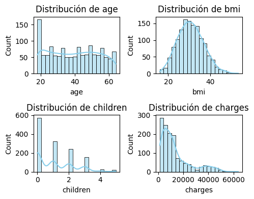

Histograma de las 4 variable numericas

fig, axes = plt.subplots(1, 3, figsize=(12,4))

for ax, col in zip(axes, categoricas):
    sns.countplot(x=col, data=df, ax=ax, hue=col)
    ax.set_title(f'Distribución de {col}')
    ax.set_xlabel(col)
    ax.set_ylabel('Frecuencia')

plt.tight_layout();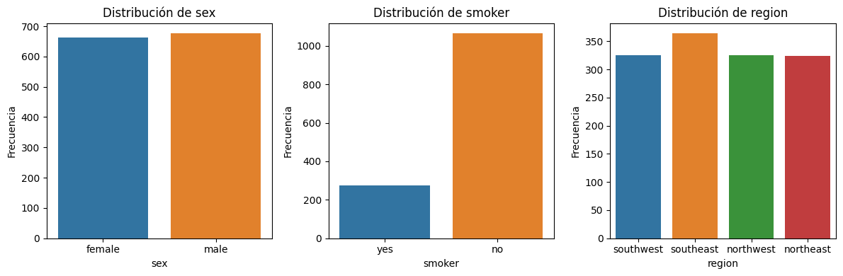

Distribución de las 3 variables categoricas

fig, axes = plt.subplots(1, 3, figsize=(16,4))

for ax, col in zip(axes, categoricas):
    sns.histplot(data=df, x='charges', hue=col, multiple='stack', ax=ax, bins=20)
    ax.set_title(f'Distribución de charges por {col}')
    ax.set_xlabel('charges')
    ax.set_ylabel('Frecuencia')

plt.tight_layout();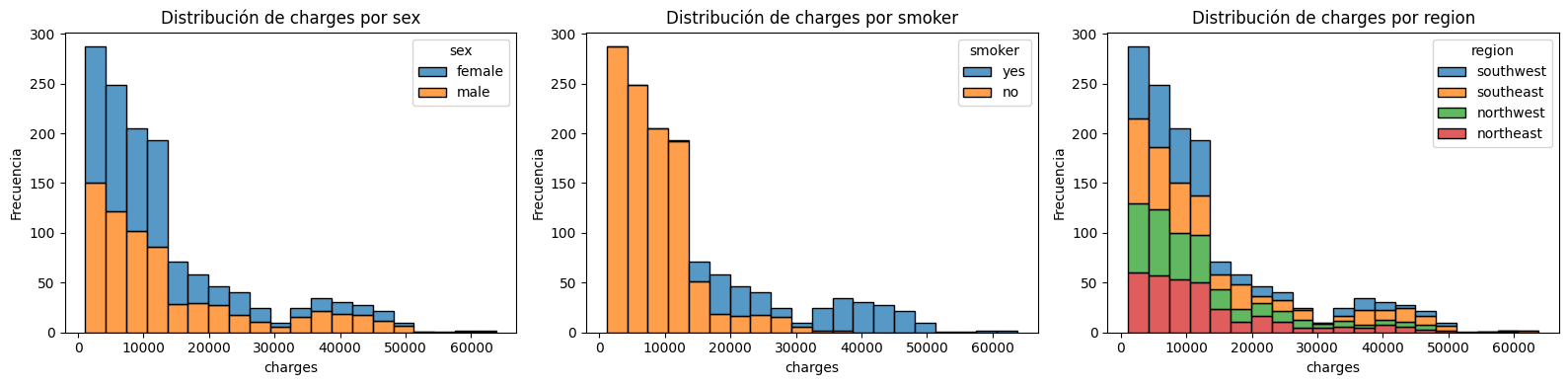

Distribución de charges para cada variable categórica

3 Tratamiento de valores outliers

Se utilizo el metodo de Winsorizing

def winsorize_series(s, factor=1.5):
    Q1, Q3 = s.quantile([0.25, 0.75])
    IQR = Q3 - Q1
    lower, upper = Q1 - factor * IQR, Q3 + factor * IQR
    return s.clip(lower, upper)

cols = ["age", "bmi", "children"]

df_original = df[cols].copy()

df_winsor = df_original.copy()
for col in cols:
    df_winsor[col] = winsorize_series(df_original[col])


fig, axes = plt.subplots(1, len(cols), figsize=(18, 5))

for i, col in enumerate(cols):
    df_compare = pd.DataFrame({
        "Valores": pd.concat([df_original[col], df_winsor[col]], ignore_index=True),
        "Estado": ["Original"] * len(df_original) + ["Winsorized"] * len(df_winsor)
    })

    sns.boxplot(data=df_compare, x="Estado", y="Valores", hue="Estado",
                palette="Set2", dodge=False, ax=axes[i])
    axes[i].set_title(f"{col} (Original vs Winsorized)", fontsize=12)
    axes[i].set_xlabel(col)

plt.suptitle("Original vs Winsorizing ", fontsize=14)
plt.tight_layout();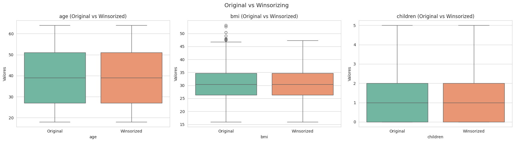

El metodo winsorizing reduce los valores extremos y ayuda a reduce la dispersión

sns.boxplot(data=df, y="charges", hue="smoker").set_title("Costo: Fumadores vs No Fumadores");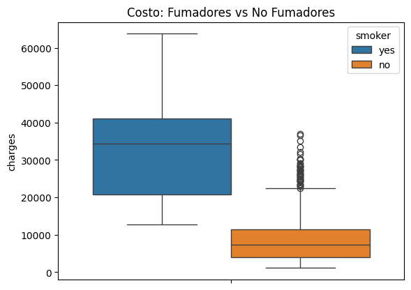

Existe un desbalance el variable smoker, el cual se debe de tomar encuenta en el modelo

4 Preprocesamiento

numericas = numericas[:-1]

X = df.drop("charges", axis=1)
y = df["charges"]

for col in numericas:
    X[col] = winsorize_series(X[col])

preproc = ColumnTransformer([
    ("num", StandardScaler(), numericas),
    ("cat", OneHotEncoder(handle_unknown="ignore", sparse_output=False), categoricas)
])

X_train, X_test, y_train, y_test = train_test_split(
    X, y, test_size=0.2, random_state=42, stratify=df["smoker"])

preproc.fit(X_train)
X_train_processed = preproc.transform(X_train)
X_test_processed = preproc.transform(X_test)

Se separo las columnas de la variable objetivo

Se redujeron los valores outliers.

Se reescalo la variables numericas.

Se transformaron las variables categorias.

Se dividio el dataset en 80% train y 20% test, se tomo encuenta en desbalance de la columna smoker, para tener una mejor distribución de los datos.

5 Selección de los modelos

modelos = {
    "linreg": LinearRegression(),
    "ridge": Ridge(random_state=42),
    "lasso": Lasso(random_state=42),
    "enet": ElasticNet(random_state=42),
    "dt": DecisionTreeRegressor(random_state=42),
    "rf": RandomForestRegressor(random_state=42, n_jobs=-1),
    "gb": GradientBoostingRegressor(random_state=42),
    "et": ExtraTreesRegressor(random_state=42, n_jobs=-1),
    "hgb": HistGradientBoostingRegressor(random_state=42),
    "knn": KNeighborsRegressor(),
    "bayes_ridge": BayesianRidge(),
    "ard": ARDRegression()
}

resultados_default = {}
for name, modelo in modelos.items():
    modelo.fit(X_train_processed, y_train)
    y_pred = modelo.predict(X_test_processed)
    resultados_default[name] = {
        "RMSE": root_mean_squared_error(y_test, y_pred),
        "MAE": mean_absolute_error(y_test, y_pred),
        "R2": r2_score(y_test, y_pred),
        "MAPE": np.mean(np.abs((y_test - y_pred) / y_test)) * 100
    }

df_resultados = pd.DataFrame(resultados_default).round(3).transpose().sort_values("RMSE")

frecuentistas = [n for n in df_resultados.index if n not in ["bayes_ridge", "ard"]]
bayesianos = ["bayes_ridge", "ard"]

print("\n--- Ranking Frecuentistas ---")
print(df_resultados.loc[frecuentistas])

--- Ranking Frecuentistas ---
            RMSE       MAE     R2    MAPE
gb      4275.516  2401.829  0.876  28.568
hgb     4719.726  2856.109  0.849  37.770
rf      4758.837  2811.406  0.846  37.836
et      5150.095  2746.673  0.820  40.756
lasso   5578.435  3873.742  0.789  38.435
ridge   5578.495  3877.731  0.789  38.492
linreg  5578.582  3873.931  0.789  38.438
knn     5964.791  3701.869  0.759  40.099
dt      6022.786  2790.782  0.754  36.124
enet    8278.938  6163.192  0.535  90.716

Se entreno con varios modelos, tanto modelos frecuentistas como bayesianos y se hizo la comparacion con la metrica RMSE

print("\n--- Top 3 Modelos Frecuentistas ---")
print(df_resultados.loc[frecuentistas][:3].sort_values("RMSE"))

print("\n---------------")

print("\n--- Modelos Bayesianos ---")
print(df_resultados.loc[bayesianos].sort_values("RMSE"))

--- Top 3 Modelos Frecuentistas ---
         RMSE       MAE     R2    MAPE
gb   4275.516  2401.829  0.876  28.568
hgb  4719.726  2856.109  0.849  37.770
rf   4758.837  2811.406  0.846  37.836

---------------

--- Modelos Bayesianos ---
                 RMSE       MAE     R2    MAPE
ard          5575.852  3865.231  0.789  38.549
bayes_ridge  5578.494  3877.773  0.789  38.493

Los modelos frecuentistas selecionados por tener menor RMSE son:

GradientBoostingRegressor
HistGradientBoostingRegressor
RandomForestRegressor

Los modelos bayesianos selecionados por tener menor RMSE son:

ARDRegression
BayesianRidge

6 Tuning los top 3 modelos frecuencistas

param_grid = {
    "ridge": {"alpha": [0.1, 1.0, 10.0]},
    "lasso": {"alpha": [0.001, 0.01, 0.1, 1.0]},
    "enet": {"alpha": [0.001, 0.01, 0.1], "l1_ratio": [0.2, 0.5, 0.8]},
    "dt": {"max_depth": [None, 5, 10, 20]},
    "rf": {"n_estimators": [200, 500], "max_depth": [None, 10, 20]},
    "gb": {"n_estimators": [100, 200], "learning_rate": [0.05, 0.1]},
    "et": {"n_estimators": [200, 500], "max_depth": [None, 10, 20]},
    "hgb": {"max_iter": [200, 500], "learning_rate": [0.05, 0.1]},
    "knn": {"n_neighbors": [5, 10, 15]},
    "bayes_ridge": {"alpha_1": [1e-6, 1e-4], "alpha_2": [1e-6, 1e-4]},
    "ard": {"alpha_1": [1e-6, 1e-4], "alpha_2": [1e-6, 1e-4]}
}

best_models, best_params = {}, {}
cv = KFold(n_splits=5, shuffle=True, random_state=42)
top3 = df_resultados.index[:3].tolist()

for name in top3:
    if name not in param_grid:
        best_models[name] = modelos[name].fit(X_train_processed, y_train)
        best_params[name] = {}
    else:
        grid = GridSearchCV(modelos[name], param_grid[name], cv=cv,
                            scoring="neg_root_mean_squared_error", n_jobs=-1)
        grid.fit(X_train_processed, y_train)
        best_models[name] = grid.best_estimator_
        best_params[name] = grid.best_params_

ajustados = {}
for name, modelo in modelos.items():
    if name in best_models:
        ajustados[name] = best_models[name]
    else:
        modelo.fit(X_train_processed, y_train)
        ajustados[name] = modelo

scores_final = {
    name: root_mean_squared_error(y_test, m.predict(X_test_processed))
    for name, m in ajustados.items()
}

best_frec_name = min(frecuentistas, key=lambda n: scores_final[n])
best_bayes_name = min(bayesianos, key=lambda n: scores_final[n])

best_frec_model = ajustados[best_frec_name]
best_bayes_model = ajustados[best_bayes_name]

Se realizo un tuning de los top 3 modelos frecuentistas y bayesianos, y se selecciono el mejor de cada enfoque, luego se evaluo en el data test.

y_pred_frec = best_frec_model.predict(X_test_processed)
y_pred_bayes, _ = best_bayes_model.predict(X_test_processed, return_std=True)

result_frec = {
    "Modelo": f"Frecuentista {best_frec_name}",
    "RMSE": root_mean_squared_error(y_test, y_pred_frec),
    "MAE": mean_absolute_error(y_test, y_pred_frec),
    "R2": r2_score(y_test, y_pred_frec),
    "MAPE": np.mean(np.abs((y_test - y_pred_frec) / y_test)) * 100  
}

result_bayes = {
    "Modelo": f"Bayesiano {best_bayes_name}",
    "RMSE": root_mean_squared_error(y_test, y_pred_bayes),
    "MAE": mean_absolute_error(y_test, y_pred_bayes),
    "R2": r2_score(y_test, y_pred_bayes),
    "MAPE": np.mean(np.abs((y_test - y_pred_bayes) / y_test)) * 100    
}

df_resultados = pd.DataFrame([result_frec, result_bayes])
df_resultados.round(3)

	Modelo	RMSE	MAE	R2	MAPE
0	Frecuentista gb	4183.896	2410.873	0.881	31.138
1	Bayesiano ard	5575.852	3865.231	0.789	38.549

La mejores metricas de cada enfoque en el data test

def obtener_intervalos(model, X, y_true=None, bayesiano=False):
    if bayesiano:
        y_mean, y_std = model.predict(X, return_std=True)
        return y_mean, y_mean - 1.96*y_std, y_mean + 1.96*y_std
    y_pred = model.predict(X)
    if hasattr(model, "estimators_") and hasattr(model, "n_estimators") and not model.__class__.__name__.startswith("GradientBoosting"):
        estimators = model.estimators_
        if isinstance(estimators, np.ndarray):
            estimators = estimators.ravel().tolist()
        member_preds = np.stack([est.predict(X) for est in estimators], axis=1)
        std_preds = member_preds.std(axis=1)
        return y_pred, y_pred - 1.96*std_preds, y_pred + 1.96*std_preds
    resid_std = np.std(y_true - y_pred)
    return y_pred, y_pred - 1.96*resid_std, y_pred + 1.96*resid_std

y_center_frec, ci_lower_frec, ci_upper_frec = obtener_intervalos(best_frec_model, X_test_processed, y_test, bayesiano=False)
y_center_bayes, ci_lower_bayes, ci_upper_bayes = obtener_intervalos(best_bayes_model, X_test_processed, bayesiano=True)

Se crean los intervalos de confianza/credibilidad de cada enfoque

7 Gráficos

Valores reales vs los predichos de cada enfoque, con su respectivo intervalo de confianza/credibilidad

sns.set_style("whitegrid")

plt.figure(figsize=(14,6))

# Frecuentista
plt.subplot(1,2,1)
sns.scatterplot(x=y_test, y=y_center_frec, hue=X_test["smoker"],
                palette={"yes":"tab:red","no":"tab:blue"}, alpha=0.6, s=35)
plt.plot([y_test.min(), y_test.max()], [y_test.min(), y_test.max()],
         color="black", linestyle="--", label="Línea identidad")
order_f = np.argsort(y_test.values)
plt.fill_between(y_test.values[order_f], ci_lower_frec[order_f], ci_upper_frec[order_f],
                 color="gray", alpha=0.3, label="IC 95%")
plt.title(f"Frecuentista: {best_frec_name}")
plt.xlabel("Valores reales")
plt.ylabel("Predicciones")
plt.legend()

# Bayesiano
plt.subplot(1,2,2)
sns.scatterplot(x=y_test, y=y_center_bayes, hue=X_test["smoker"],
                palette={"yes":"tab:red","no":"tab:blue"}, alpha=0.6, s=35)
plt.plot([y_test.min(), y_test.max()], [y_test.min(), y_test.max()],
         color="black", linestyle="--", label="Línea identidad")
order_b = np.argsort(y_test.values)
plt.fill_between(y_test.values[order_b], ci_lower_bayes[order_b], ci_upper_bayes[order_b],
                 color="gray", alpha=0.3, label="IC 95% (credibilidad)")
plt.title(f"Bayesiano: {best_bayes_name}")
plt.xlabel("Valores reales")
plt.ylabel("Predicciones")
plt.legend()

plt.tight_layout();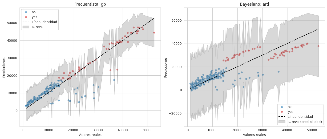

Se observa que el modelo frecuentista predice mejor, ademas de ver que los no fumadores causan mayor problema para la prediccion por los valores outliers que tienen

resid_frec = y_test.values - y_center_frec
resid_bayes = y_test.values - y_center_bayes
band_frec = (ci_upper_frec - y_center_frec)
band_bayes = (ci_upper_bayes - y_center_bayes)

plt.figure(figsize=(14,6))


plt.subplot(1,2,1)
sns.scatterplot(x=y_center_frec, y=resid_frec, hue=X_test["smoker"],
                palette={"yes":"tab:red","no":"tab:blue"}, alpha=0.6, s=35)
plt.axhline(0, color="black", linestyle="--", label="Cero")
order_rf = np.argsort(y_center_frec)
plt.fill_between(y_center_frec[order_rf], -band_frec[order_rf], band_frec[order_rf],
                 color="gray", alpha=0.3, label="IC 95% aprox.")
plt.title(f"Residuales Frecuentista: {best_frec_name}")
plt.xlabel("Predicciones")
plt.ylabel("Residuales")
plt.legend()


plt.subplot(1,2,2)
sns.scatterplot(x=y_center_bayes, y=resid_bayes, hue=X_test["smoker"],
                palette={"yes":"tab:red","no":"tab:blue"}, alpha=0.6, s=35)
plt.axhline(0, color="black", linestyle="--", label="Cero")
order_rb = np.argsort(y_center_bayes)
plt.fill_between(y_center_bayes[order_rb], -band_bayes[order_rb], band_bayes[order_rb],
                 color="gray", alpha=0.3, label="IC 95% (credibilidad)")
plt.title(f"Residuales Bayesiano: {best_bayes_name}")
plt.xlabel("Predicciones")
plt.ylabel("Residuales")
plt.legend()

plt.tight_layout();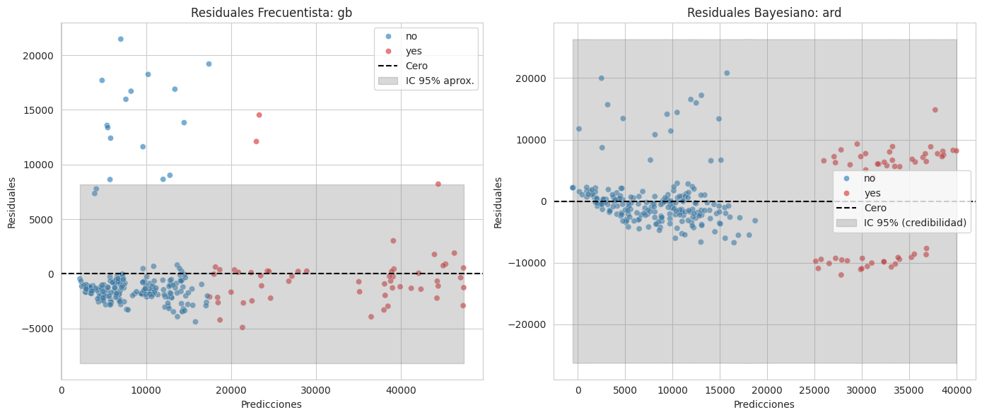

Se observa lo mismo con los gráficos de los residuos

8 SHAP

Varibles Explicativas para el modelo Frecuentista

feature_names = preproc.get_feature_names_out().tolist()
explainer_frec = shap.Explainer(best_frec_model, X_train_processed)
shap_values_frec = explainer_frec(X_test_processed)


plt.title(f"SHAP Summary - {best_frec_name}")
shap.summary_plot(shap_values_frec, X_test_processed, feature_names=feature_names)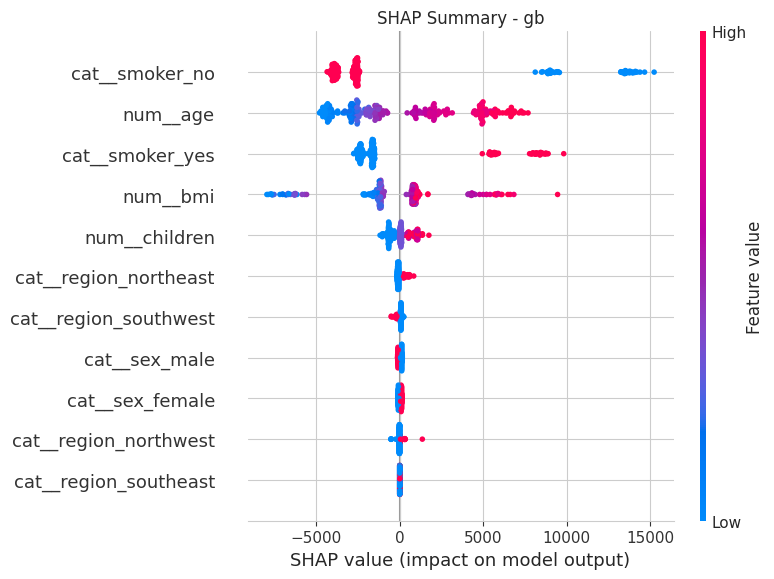

El SHAP de gb muestra que la varible no fumadores tiene un gran impacto, seguido de los fumadores en la variable charges

Varibles Explicativas para el modelo Bayesiano

explainer_bayes = shap.Explainer(best_bayes_model, X_train_processed)
shap_values_bayes = explainer_bayes(X_test_processed)

plt.title(f"SHAP Summary - {best_bayes_name}")
shap.summary_plot(shap_values_bayes, X_test_processed, feature_names=feature_names)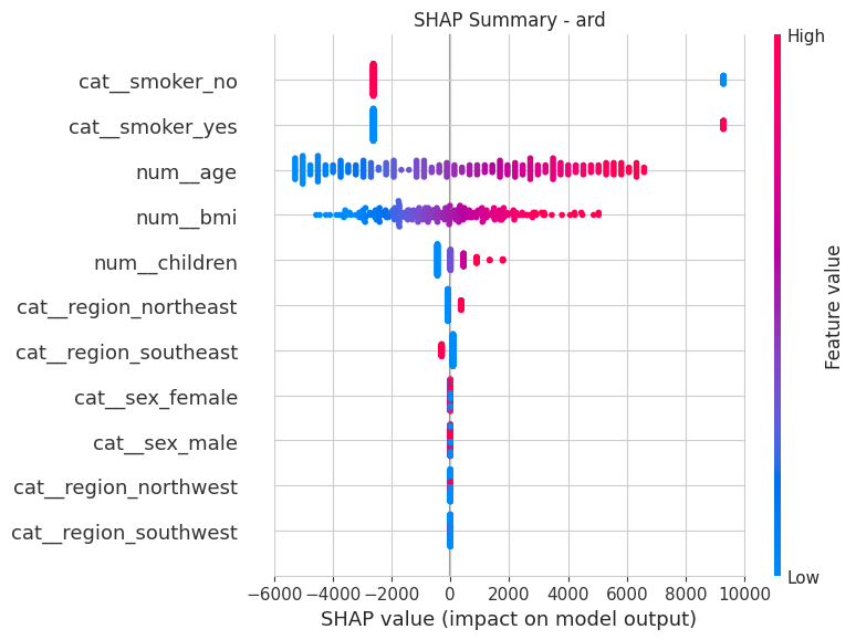

9 Guardar modelo

Se guarda el modelo el formato onnx para ser ejecutado en la web o móvil

n_features = X_train_processed.shape[1]
initial_type = [('float_input', FloatTensorType([None, n_features]))]

onnx_frec = convert_sklearn(best_frec_model,
                            target_opset=13,  
                            initial_types=initial_type)
with open("best_frec_model.onnx", "wb") as f:
    f.write(onnx_frec.SerializeToString())

onnx_bayes = convert_sklearn(best_bayes_model, 
                             target_opset=13, 
                             initial_types=initial_type)
with open("best_bayes_model.onnx", "wb") as f:
    f.write(onnx_bayes.SerializeToString())

Verificar si el modelo se guardo correctamente a traves de la introducción de un dato

sess_frec = ort.InferenceSession("best_frec_model.onnx")
sess_bayes = ort.InferenceSession("best_bayes_model.onnx")

sample_input = X_test_processed[0:1].astype(np.float32)
input_name_frec = sess_frec.get_inputs()[0].name
input_name_bayes = sess_bayes.get_inputs()[0].name

pred_frec = sess_frec.run(None, {input_name_frec: sample_input})[0]
pred_bayes = sess_bayes.run(None, {input_name_bayes: sample_input})[0]

print("Predicción Frecuentista:", pred_frec)
print("Predicción Bayesiana:", pred_bayes)

print("Valor real de test:", y_test.iloc[0])

Predicción Frecuentista: [[8627.369]]
Predicción Bayesiana: [[7778.1484]]
Valor real de test: 6799.458

Valores de las columnas X’s

print("Valor real de test:\n", X_test.iloc[0])

Valor real de test:
 age                31
sex              male
bmi              28.5
children            5
smoker             no
region      northeast
Name: 71, dtype: object